Singular Value Decompositions

Thomas E. Baker—August 19, 2015

A singular value decomposition (SVD) can be computed for any rectangular matrix. The properties of this decomposition allows us to sort out relevant "degrees of freedom" and only keep the most important parts of the matrix. Leaving out the less important degrees of freedom in a DMRG calculation, for example, allows it to go much faster by working with smaller matrices (for one-dimensional systems reducing the cost from exponential down to roughly linear!). Often, the degrees of freedom we throw away are very small and don't affect the final answer.

This article will explain what the SVD is, how to represent it diagrammatically, and how to compute it in ITensor.

Singular Value Decompositions

The singular value decomposition of a matrix @@M@@ is a factorization @@M = U D V^\dagger@@ where @@U@@ and @@V@@ are unitary, and @@D@@ is diagonal, with real, non-negative entries (known as the singular values).

Consider a rectangular matrix (this is coded in the first Tutorial)

The singular value decomposition of @@M@@ is

Thus for this matrix the singular values are 0.933, 0.300, and 0.200. Observe that @@MM^\dagger=UD^2U^\dagger@@ , so we can see the singular values are the square roots of the eigenvalues of @@M M^\dagger @@ (which is by construction Hermitian and positive semi-definite).

The real utility of the SVD is that it provides a controlled method for approximating matrices. For instance, if we set the smallest singular value to zero, then

Since we set the third singular value to zero, we can now safely truncate (discard) the third column of @@U@@ and the third row of @@V^\dagger@@ without affecting the result @@\tilde{M}@@

Even though the values of the modified matrix have changed, the norm of the difference, @@||M-\tilde M||^2=0.04=(0.2)^2@@ . Note that the value is not large and does a good job of approximating the original matrix, and we get to leave off the rows and columns corresponding to the truncated values.

The error we calculated above is related to the truncation error in a DMRG calculation, defined as the sum of the squares of the singular values that we neglect when compressing the wavefunction. In the DMRG case, these singular values can go very low, very nearly zero, and leaving them out of the SVD produces almost no change in the wavefunction.

Diagrammatically

Consider a two site wavefunction

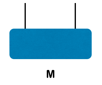
The SVD can be represented diagramatically as

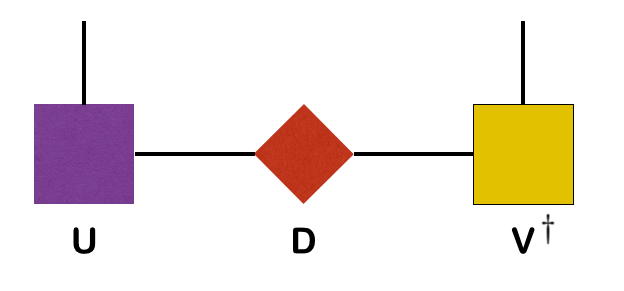
In ITensor

To compute an svd in ITensor, we can use the code

Index i1,i2,i3,i4;
//...initialize i1,i2,i3,i4...
ITensor T(i1,i2,i3,i4);
//...initialize T...
ITensor U(i1,i3),D,V;
svd(T,U,D,V);

The first argument is the tensor T we want to decompose, which can have any number of indices. Because the SVD is a matrix (rank 2 tensor) decomposition, we must specify which indices of T are to be combined into a collective "row" index; the rest will be combined into the "column" index.

To specify which indices end up on U (the "row" indices), initialize U to have these indices. Any indices of U shared with T will still be on U when the SVD is done; all remaining indices of T will appear on V. (If U has no indices, V is inspected instead.) Indices initially on U and V which are not shared with T will be removed. Upon return U and V will each have a new, extra index they uniquely share with D.

To easily access the new indices D shares with U and V, use the following code

auto du = commonIndex(D,U);
auto dv = commonIndex(D,V);

After the SVD in the example above, U will have indices i1, i3, and du, while V will have indices i2, i4, and dv.

Calculating Entanglement

The von Neumann entanglement can be calculated from the expression

where each eigenvalue of the reduced density matrix, @@\rho_i@@ , is simply the square of the singular values in D. We often abbreviate the singular values as @@\lambda_i(=\sqrt{\rho_i})@@ . The density matrix eigenvalues can be accessed through the eigsKept() function of the Spectrum object returned by the svd function:

auto spectrum = svd(T,U,D,V);
Real SvN=0.;//The von Neumann entropy
for(auto eig : spectrum.eigsKept())
{
SvN += -eig * log(eig);
}